#!pip install ANNarchyHomeostatic STDP: SORF model
![]()
![]()
Reimplementation of the SORF model published in:
Carlson, K.D.; Richert, M.; Dutt, N.; Krichmar, J.L., “Biologically plausible models of homeostasis and STDP: Stability and learning in spiking neural networks,” in Neural Networks (IJCNN), The 2013 International Joint Conference on , vol., no., pp.1-8, 4-9 Aug. 2013. doi: 10.1109/IJCNN.2013.6706961
import numpy as np
import matplotlib.pyplot as plt
import ANNarchy as ann

from tqdm import tqdm
ANNarchy 5.0 (5.0.2) on linux (posix).Hyperparameters:
nb_neuron = 4 # Number of exc and inh neurons
size = (32, 32) # input size
freq = 1.2 # nb_cycles/half-image
nb_stim = 40 # Number of grating per epoch
nb_epochs = 20 # Number of epochs
max_freq = 28. # Max frequency of the poisson neurons
T = 10000. # Period for averaging the firing rate
Neuron type:
# Izhikevich Coba neuron with AMPA, NMDA and GABA receptors
RSNeuron = ann.Neuron(
    parameters = dict(
        a = 0.02,
        b = 0.2,
        c = -65.,
        d = 8.,

        tau_ampa = 5.,
        tau_nmda = 150.,
        tau_gabaa = 6.,
        tau_gabab = 150.,

        vrev_ampa = 0.0,
        vrev_nmda = 0.0,
        vrev_gabaa = -70.0,
        vrev_gabab = -90.0,
     ) ,
    equations = [
        # Inputs
        ann.Variable("""
            I = g_ampa * (vrev_ampa - v) + g_nmda * nmda(v, -80.0, 60.0) * (vrev_nmda -v) + g_gabaa * (vrev_gabaa - v) + g_gabab * (vrev_gabab -v)
        """),

        # Midpoint scheme
        ann.Variable("dv/dt = (0.04 * v + 5.0) * v + 140.0 - u + I", init=-65., min=-90., method='midpoint'),
        ann.Variable("du/dt = a * (b*v - u)", init=-13., method='midpoint'),

        # Conductances
        ann.Variable("tau_ampa * dg_ampa/dt = -g_ampa", method='exponential'),
        ann.Variable("tau_nmda * dg_nmda/dt = -g_nmda", method='exponential'),
        ann.Variable("tau_gabaa * dg_gabaa/dt = -g_gabaa", method='exponential'),
        ann.Variable("tau_gabab * dg_gabab/dt = -g_gabab", method='exponential'),
    ],
    spike = "v >= 30.",
    reset = """
        v = c
        u += d
        g_ampa = 0.0
        g_nmda = 0.0
        g_gabaa = 0.0
        g_gabab = 0.0
    """,
    functions = """
        nmda(v, t, s) = ((v-t)/(s))^2 / (1.0 + ((v-t)/(s))^2)
    """,
    refractory=1.0
)
Synapse:
# STDP with homeostatic regulation
homeo_stdp = ann.Synapse(
    parameters=dict(
        # STDP
        tau_plus  = 60.,
        tau_minus = 90.,
        A_plus  = 0.000045,
        A_minus = 0.00003,

        # Homeostatic regulation
        alpha = 0.1,
        beta = 50.0, # <- Difference with the original implementation
        gamma = 50.0,
        Rtarget = 10.,
        T = 10000.,
    ),
    equations = [
        # Homeostatic values
        ann.Variable("R = post.r", locality='semiglobal'),
        ann.Variable("K = R/(T * (1. + fabs(1. - R / Rtarget) * gamma))", locality='semiglobal'),

        # Nearest-neighbour
        ann.Variable("stdp = if t_post >= t_pre: ltp else: - ltd"),
        ann.Variable("w += (alpha * w * (1- R/Rtarget) + beta * stdp ) * K", min=0.0, max=10.0),

        # Traces
        ann.Variable("tau_plus  * dltp/dt = -ltp", method="exponential"),
        ann.Variable("tau_minus * dltd/dt = -ltd", method="exponential"),
    ],
    pre_spike="""
        g_target += w
        ltp = A_plus
    """,
    post_spike="ltd = A_minus"
)
Network:
# Network
net = ann.Network()

# Input population
OnPoiss = net.create(ann.PoissonPopulation(size, rates=1.0))
OffPoiss = net.create(ann.PoissonPopulation(size, rates=1.0))

# RS neuron for the input buffers
OnBuffer = net.create(size, RSNeuron)
OffBuffer = net.create(size, RSNeuron)

# Connect the buffers
OnPoissBuffer = net.connect(OnPoiss, OnBuffer, ['ampa', 'nmda'])
OnPoissBuffer.one_to_one(ann.Uniform(0.2, 0.6))
OffPoissBuffer = net.connect(OffPoiss, OffBuffer, ['ampa', 'nmda'])
OffPoissBuffer.one_to_one(ann.Uniform(0.2, 0.6))

# Excitatory and inhibitory neurons
Exc = net.create(nb_neuron, RSNeuron)
Inh = net.create(nb_neuron, RSNeuron)
Exc.compute_firing_rate(T)
Inh.compute_firing_rate(T)

# Input connections
OnBufferExc = net.connect(OnBuffer, Exc, ['ampa', 'nmda'], homeo_stdp)
OnBufferExc.all_to_all(ann.Uniform(0.004, 0.015))
OffBufferExc = net.connect(OffBuffer, Exc, ['ampa', 'nmda'], homeo_stdp)
OffBufferExc.all_to_all(ann.Uniform(0.004, 0.015))

# Competition
ExcInh = net.connect(Exc, Inh, ['ampa', 'nmda'], homeo_stdp)
ExcInh.all_to_all(ann.Uniform(0.116, 0.403))

ExcInh.Rtarget = 75.
ExcInh.tau_plus = 51.
ExcInh.tau_minus = 78.
ExcInh.A_plus = -0.000041
ExcInh.A_minus = -0.000015

InhExc = net.connect(Inh, Exc, ['gabaa', 'gabab'])
InhExc.all_to_all(ann.Uniform(0.065, 0.259))

net.compile()
Compiling network 1... OK# Inputs
def get_grating(theta):
x = np.linspace(-1., 1., size[0])
y = np.linspace(-1., 1., size[1])
xx, yy = np.meshgrid(x, y)
z = np.sin(2.*np.pi*(np.cos(theta)*xx + np.sin(theta)*yy)*freq)
return np.maximum(z, 0.), -np.minimum(z, 0.0)
# Initial weights
w_on_start = OnBufferExc.w
w_off_start = OffBufferExc.w
# Monitors
m = net.monitor(Exc, 'r')
n = net.monitor(Inh, 'r')
o = net.monitor(OnBufferExc[0], 'w', period=1000.)
p = net.monitor(ExcInh[0], 'w', period=1000.)
# Learning procedure
from time import time
import random
tstart = time()
stim_order = list(range(nb_stim))
for epoch in tqdm(range(nb_epochs)):
random.shuffle(stim_order)
for stim in stim_order:
# Generate a grating randomly
rates_on, rates_off = get_grating(np.pi*stim/float(nb_stim))
# Set it as input to the poisson neurons
OnPoiss.rates = max_freq * rates_on
OffPoiss.rates = max_freq * rates_off
# Simulate for 2s
net.simulate(2000.)
# Relax the Poisson inputs
OnPoiss.rates = 1.
OffPoiss.rates = 1.
# Simulate for 500ms
net.simulate(500.)
print('Done in ', time()-tstart)
# Recordings
datae = m.get('r')
datai = n.get('r')
dataw = o.get('w')
datal = p.get('w') 0%| | 0/20 [00:00<?, ?it/s] 5%|████ | 1/20 [00:11<03:40, 11.61s/it] 10%|████████▏ | 2/20 [00:23<03:29, 11.65s/it] 15%|████████████▎ | 3/20 [00:34<03:17, 11.61s/it] 20%|████████████████▍ | 4/20 [00:46<03:05, 11.57s/it] 25%|████████████████████▌ | 5/20 [00:57<02:53, 11.59s/it] 30%|████████████████████████▌ | 6/20 [01:09<02:42, 11.64s/it] 35%|████████████████████████████▋ | 7/20 [01:21<02:31, 11.69s/it] 40%|████████████████████████████████▊ | 8/20 [01:33<02:23, 11.93s/it] 45%|████████████████████████████████████▉ | 9/20 [01:46<02:12, 12.04s/it]WARNING: The recording of monitors might consume 116MiB, i.e. more then 10% of your currently available memory.
WARNING: Please note, that estimate considers only recorded state variables. Other attributes, such as spike recordings, are not included. 50%|████████████████████████████████████████▌ | 10/20 [01:57<01:59, 11.95s/it]WARNING: The recording of monitors might consume 117MiB, i.e. more then 10% of your currently available memory.
WARNING: The recording of monitors might consume 118MiB, i.e. more then 10% of your currently available memory.
WARNING: The recording of monitors might consume 119MiB, i.e. more then 10% of your currently available memory.
WARNING: The recording of monitors might consume 120MiB, i.e. more then 10% of your currently available memory.
WARNING: The recording of monitors might consume 168MiB, i.e. more then 10% of your currently available memory.
WARNING: The recording of monitors might consume 169MiB, i.e. more then 10% of your currently available memory.
WARNING: The recording of monitors might consume 170MiB, i.e. more then 10% of your currently available memory.
WARNING: The recording of monitors might consume 171MiB, i.e. more then 10% of your currently available memory. 55%|████████████████████████████████████████████▌ | 11/20 [02:09<01:47, 11.96s/it]WARNING: The recording of monitors might consume 172MiB, i.e. more then 10% of your currently available memory.
WARNING: The recording of monitors might consume 173MiB, i.e. more then 10% of your currently available memory.
WARNING: The recording of monitors might consume 174MiB, i.e. more then 10% of your currently available memory.
WARNING: The recording of monitors might consume 175MiB, i.e. more then 10% of your currently available memory.
WARNING: The recording of monitors might consume 176MiB, i.e. more then 10% of your currently available memory.
WARNING: The recording of monitors might consume 177MiB, i.e. more then 10% of your currently available memory.
WARNING: The recording of monitors might consume 178MiB, i.e. more then 10% of your currently available memory. 60%|████████████████████████████████████████████████▌ | 12/20 [02:21<01:35, 11.98s/it]WARNING: The recording of monitors might consume 179MiB, i.e. more then 10% of your currently available memory.
WARNING: The recording of monitors might consume 180MiB, i.e. more then 10% of your currently available memory.
WARNING: The recording of monitors might consume 181MiB, i.e. more then 10% of your currently available memory.
WARNING: The recording of monitors might consume 182MiB, i.e. more then 10% of your currently available memory.
WARNING: The recording of monitors might consume 183MiB, i.e. more then 10% of your currently available memory.
WARNING: The recording of monitors might consume 184MiB, i.e. more then 10% of your currently available memory.
WARNING: The recording of monitors might consume 185MiB, i.e. more then 10% of your currently available memory. 65%|████████████████████████████████████████████████████▋ | 13/20 [02:33<01:23, 11.96s/it]WARNING: The recording of monitors might consume 186MiB, i.e. more then 10% of your currently available memory.
WARNING: The recording of monitors might consume 187MiB, i.e. more then 10% of your currently available memory.
WARNING: The recording of monitors might consume 188MiB, i.e. more then 10% of your currently available memory.
WARNING: The recording of monitors might consume 189MiB, i.e. more then 10% of your currently available memory.
WARNING: The recording of monitors might consume 190MiB, i.e. more then 10% of your currently available memory.
WARNING: The recording of monitors might consume 191MiB, i.e. more then 10% of your currently available memory.
WARNING: The recording of monitors might consume 192MiB, i.e. more then 10% of your currently available memory. 70%|████████████████████████████████████████████████████████▋ | 14/20 [02:45<01:11, 11.93s/it]WARNING: The recording of monitors might consume 193MiB, i.e. more then 10% of your currently available memory.
WARNING: The recording of monitors might consume 194MiB, i.e. more then 10% of your currently available memory.
WARNING: The recording of monitors might consume 195MiB, i.e. more then 10% of your currently available memory.
WARNING: The recording of monitors might consume 196MiB, i.e. more then 10% of your currently available memory.
WARNING: The recording of monitors might consume 197MiB, i.e. more then 10% of your currently available memory.
WARNING: The recording of monitors might consume 198MiB, i.e. more then 10% of your currently available memory.
WARNING: The recording of monitors might consume 199MiB, i.e. more then 10% of your currently available memory. 75%|████████████████████████████████████████████████████████████▊ | 15/20 [02:57<00:59, 11.96s/it]WARNING: The recording of monitors might consume 200MiB, i.e. more then 10% of your currently available memory.
WARNING: The recording of monitors might consume 201MiB, i.e. more then 10% of your currently available memory.
WARNING: The recording of monitors might consume 202MiB, i.e. more then 10% of your currently available memory.
WARNING: The recording of monitors might consume 203MiB, i.e. more then 10% of your currently available memory.
WARNING: The recording of monitors might consume 204MiB, i.e. more then 10% of your currently available memory.
WARNING: The recording of monitors might consume 205MiB, i.e. more then 10% of your currently available memory.
WARNING: The recording of monitors might consume 206MiB, i.e. more then 10% of your currently available memory. 80%|████████████████████████████████████████████████████████████████▊ | 16/20 [03:09<00:47, 11.97s/it]WARNING: The recording of monitors might consume 207MiB, i.e. more then 10% of your currently available memory.
WARNING: The recording of monitors might consume 208MiB, i.e. more then 10% of your currently available memory.
WARNING: The recording of monitors might consume 209MiB, i.e. more then 10% of your currently available memory.
WARNING: The recording of monitors might consume 210MiB, i.e. more then 10% of your currently available memory.
WARNING: The recording of monitors might consume 211MiB, i.e. more then 10% of your currently available memory.
WARNING: The recording of monitors might consume 212MiB, i.e. more then 10% of your currently available memory.
WARNING: The recording of monitors might consume 213MiB, i.e. more then 10% of your currently available memory. 85%|████████████████████████████████████████████████████████████████████▊ | 17/20 [03:21<00:36, 12.04s/it]WARNING: The recording of monitors might consume 214MiB, i.e. more then 10% of your currently available memory.
WARNING: The recording of monitors might consume 215MiB, i.e. more then 10% of your currently available memory.
WARNING: The recording of monitors might consume 216MiB, i.e. more then 10% of your currently available memory.
WARNING: The recording of monitors might consume 217MiB, i.e. more then 10% of your currently available memory.
WARNING: The recording of monitors might consume 218MiB, i.e. more then 10% of your currently available memory.
WARNING: The recording of monitors might consume 219MiB, i.e. more then 10% of your currently available memory. 90%|████████████████████████████████████████████████████████████████████████▉ | 18/20 [03:34<00:24, 12.08s/it]WARNING: The recording of monitors might consume 220MiB, i.e. more then 10% of your currently available memory.
WARNING: The recording of monitors might consume 221MiB, i.e. more then 10% of your currently available memory.
WARNING: The recording of monitors might consume 222MiB, i.e. more then 10% of your currently available memory.
WARNING: The recording of monitors might consume 223MiB, i.e. more then 10% of your currently available memory.
WARNING: The recording of monitors might consume 224MiB, i.e. more then 10% of your currently available memory.
WARNING: The recording of monitors might consume 225MiB, i.e. more then 10% of your currently available memory.
WARNING: The recording of monitors might consume 226MiB, i.e. more then 10% of your currently available memory. 95%|████████████████████████████████████████████████████████████████████████████▉ | 19/20 [03:46<00:12, 12.10s/it]WARNING: The recording of monitors might consume 227MiB, i.e. more then 10% of your currently available memory.
WARNING: The recording of monitors might consume 228MiB, i.e. more then 10% of your currently available memory.
WARNING: The recording of monitors might consume 229MiB, i.e. more then 10% of your currently available memory.
WARNING: The recording of monitors might consume 230MiB, i.e. more then 10% of your currently available memory.
WARNING: The recording of monitors might consume 231MiB, i.e. more then 10% of your currently available memory.
WARNING: The recording of monitors might consume 232MiB, i.e. more then 10% of your currently available memory.
WARNING: The recording of monitors might consume 233MiB, i.e. more then 10% of your currently available memory. 100%|█████████████████████████████████████████████████████████████████████████████████| 20/20 [03:57<00:00, 11.94s/it]100%|█████████████████████████████████████████████████████████████████████████████████| 20/20 [03:57<00:00, 11.89s/it]Done in 237.85921263694763# Final weights
w_on_end = OnBufferExc.w
w_off_end = OffBufferExc.w
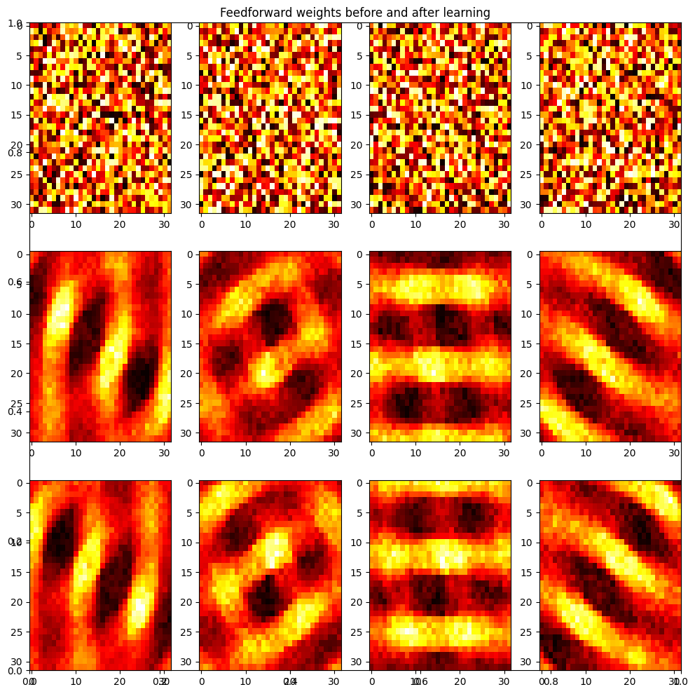
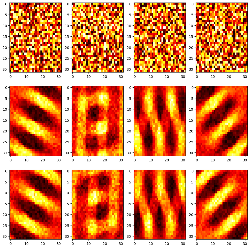
# Plot
plt.figure(figsize=(12, 12))
plt.title('Feedforward weights before and after learning')
for i in range(nb_neuron):
plt.subplot(3, nb_neuron, i+1)
plt.imshow((np.array(w_on_start[i])).reshape((32,32)), aspect='auto', cmap='hot')
plt.subplot(3, nb_neuron, nb_neuron + i +1)
plt.imshow((np.array(w_on_end[i])).reshape((32,32)), aspect='auto', cmap='hot')
plt.subplot(3, nb_neuron, 2*nb_neuron + i +1)
plt.imshow((np.array(w_off_end[i])).reshape((32,32)), aspect='auto', cmap='hot')
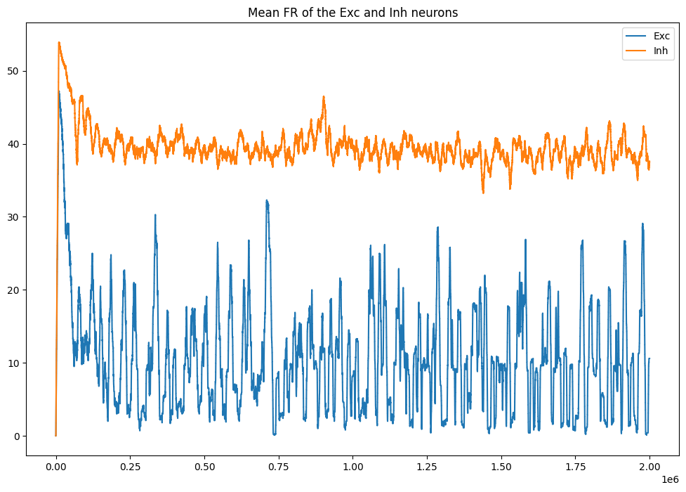
plt.figure(figsize=(12, 8))
plt.plot(datae[:, 0], label='Exc')
plt.plot(datai[:, 0], label='Inh')
plt.title('Mean FR of the Exc and Inh neurons')
plt.legend()
plt.figure(figsize=(12, 8))
plt.subplot(121)
plt.imshow(np.array(dataw, dtype='float').T, aspect='auto', cmap='hot')
plt.title('Timecourse of feedforward weights')
plt.colorbar()
plt.subplot(122)
plt.imshow(np.array(datal, dtype='float').T, aspect='auto', cmap='hot')
plt.title('Timecourse of inhibitory weights')
plt.colorbar()
plt.show()