Izhikevich’s pulse-coupled network

#!pip install ANNarchy

This script reproduces the simple pulse-coupled network proposed by Eugene Izhikevich in the article:

Izhikevich, E.M. (2003). Simple Model of Spiking Neurons, IEEE Transaction on Neural Networks, 14:6.

import numpy as np
import matplotlib.pyplot as plt

import ANNarchy as ann
ann.clear()

ANNarchy 4.8 (4.8.2) on darwin (posix).

The original Matlab code is provided below:

% Created by Eugene M. Izhikevich, February 25, 2003
% Excitatory neurons Inhibitory neurons
Ne = 800; Ni = 200;
re = rand(Ne,1); ri = rand(Ni,1);
a = [0.02*ones(Ne,1); 0.02+0.08*ri];
b = [0.2*ones(Ne,1); 0.25-0.05*ri];
c = [-65+15*re.^2; -65*ones(Ni,1)];
d = [8-6*re.^2; 2*ones(Ni,1)];
S = [0.5*rand(Ne+Ni,Ne), -rand(Ne+Ni,Ni)];
v = -65*ones(Ne+Ni,1); % Initial values of v
u = b.*v; % Initial values of u
firings = []; % spike timings
for t=1:1000 % simulation of 1000 ms
    I = [5*randn(Ne,1);2*randn(Ni,1)]; % thalamic input
    fired = find(v>=30); % indices of spikes
    firings = [firings; t+0*fired,fired];
    v(fired) = c(fired);
    u(fired) = u(fired) + d(fired);
    I = I + sum(S(:,fired),2);
    v = v + 0.5*(0.04*v.^2 + 5*v + 140 - u + I); % step 0.5 ms
    v = v + 0.5*(0.04*v.^2 + 5*v + 140-u + I); % for numerical
    u = u + a.*(b.*v - u); % stability
end;
plot(firings(:,1),firings(:,2),’.’)

Neuron type

The network is composed of parameterized quadratic integrate-and-fire neurons, known as Izhikevich neurons. They are simply defined by the following equations:

\frac{dv(t)}{dt} = 0.04 \, v^2(t) + 5 \, v(t) + 140 - u(t) + I(t)

\frac{du(t)}{dt} = a \, (b \, v(t) - u)

with v(t) representing the membrane potential and u(t) the recovery variable. The spiking mechanism is defined by a threshold on v(t), so that it emits a spike when it exceeds V_T = 30 mV. The membrane potential is reset to c and the recovery variable is incremented from d

\text{if} \; v(t) > V_T : \; \begin{cases} \text{emit a spike} \\ v(t) \leftarrow c \\ u(t) \leftarrow u(t) + d \\ \end{cases}

a, b, c, d are parameters allowing to reproduce many types of neural firing.

I(t) is the input voltage to a neuron at each time step t. For the desired network, it is the sum of a random value taken from a normal distribution with mean 0.0 and variance 1.0 (multiplied by a scaling factor) and the net effect of incoming spikes (excitatory and inhibitory).

Implementing such a neuron in ANNarchy is straightforward:

Izhikevich = ann.Neuron(
    parameters="""
        noise = 5.0 
        a = 0.02
        b = 0.2
        c = -65.0
        d = 2.0 
        v_thresh = 30.0
    """,
    equations="""
        # Input current
        I = g_exc - g_inh + noise * Normal(0.0, 1.0)

        # Membrane potential
        dv/dt = 0.04 * v^2 + 5.0 * v + 140.0 - u + I 

        # Recovery variable
        du/dt = a * (b*v - u) 
    """,
    spike = """
        v >= v_thresh
    """,
    reset = """
        v = c
        u += d
    """
)

The parameters a, b, c, d as well as the noise amplitude noise are declared in the parameters argument, as their value is constant during the simulation.

The equations for v and u are direct translations of their mathematical counterparts. Note the use of dx/dt for the time derivative and ^2 for the square function.

The input voltage I is defined as the sum of:

the total conductance of excitatory synapses g_exc,
the total conductance of inhibitory synapses -g_inh (in this example, we consider all weights to be positive, so we need to invert g_inh in order to model inhibitory synapses),
a random number taken from the normal distribution N(0,1) and multiplied by the noise scale noise.

In the pulse-coupled network, synapses are considered as instantaneous, i.e. a pre-synaptic spikes increases immediately the post-synaptic conductance proportionally to the weight of the synapse, but does not leave further trace. As this is the default behavior in ANNarchy, nothing has to be specified in the neuron’s equations.

The spike argument specifies the condition for when a spike should be emitted (here the membrane potential v should be greater than v_thresh). The reset argument specifies the changes to neural variables that should occur after a spike is emitted: here, the membrane potential is reset to the resting potential c and the membrane recovery variable u is increased from d.

Defining the populations

We start by defining a population of 1000 Izhikevich neurons and split it into 800 excitatory neurons and 200 inhibitory ones:

pop = ann.Population(geometry=1000, neuron=Izhikevich)

Exc = pop[:800]
Inh = pop[800:]

Exc and Inh are subsets of pop, which have the same properties as a population. We can then set parameters differently for each population:

re = np.random.random(800)      ; ri = np.random.random(200)
Exc.noise = 5.0                 ; Inh.noise = 2.0
Exc.a = 0.02                    ; Inh.a = 0.02 + 0.08 * ri
Exc.b = 0.2                     ; Inh.b = 0.25 - 0.05 * ri
Exc.c = -65.0 + 15.0 * re**2    ; Inh.c = -65.0
Exc.d = 8.0 - 6.0 * re**2       ; Inh.d = 2.0
Exc.v = -65.0                   ; Inh.v = -65.0
Exc.u = Exc.v * Exc.b           ; Inh.u = Inh.v * Inh.b

Defining the projections

We can now define the connections within the network:

The excitatory neurons are connected to all neurons with a weight randomly chosen in [0, 0.5]
The inhibitory neurons are connected to all neurons with a weight randomly chosen in [0, 1]

exc_proj = ann.Projection(pre=Exc, post=pop, target='exc')
exc_proj.connect_all_to_all(weights=ann.Uniform(0.0, 0.5))
   
inh_proj = ann.Projection(pre=Inh, post=pop, target='inh')
inh_proj.connect_all_to_all(weights=ann.Uniform(0.0, 1.0))

<ANNarchy.core.Projection.Projection at 0x127c3b9b0>

The network is now ready, we can compile:

ann.compile()

Compiling ...  OK

Running the simulation

We start by monitoring the spikes and membrane potential in the whole population:

m = ann.Monitor(pop, ['spike', 'v'])

We run the simulation for 1000 milliseconds:

ann.simulate(1000.0, measure_time=True)

Simulating 1.0 seconds of the network took 0.038668155670166016 seconds.

We retrieve the recordings, generate a raster plot and the population firing rate:

spikes = m.get('spike')
v = m.get('v')
t, n = m.raster_plot(spikes)
fr = m.histogram(spikes)

We plot:

The raster plot of population
The evolution of the membrane potential of a single excitatory neuron
The population firing rate

plt.figure(figsize=(12, 12))

# First plot: raster plot
plt.subplot(311)
plt.plot(t, n, 'b.')
plt.title('Raster plot')

# Second plot: membrane potential of a single excitatory cell
plt.subplot(312)
plt.plot(v[:, 15]) # for example
plt.title('Membrane potential')

# Third plot: number of spikes per step in the population.
plt.subplot(313)
plt.plot(fr)
plt.title('Number of spikes')
plt.xlabel('Time (ms)')

plt.tight_layout()
plt.show()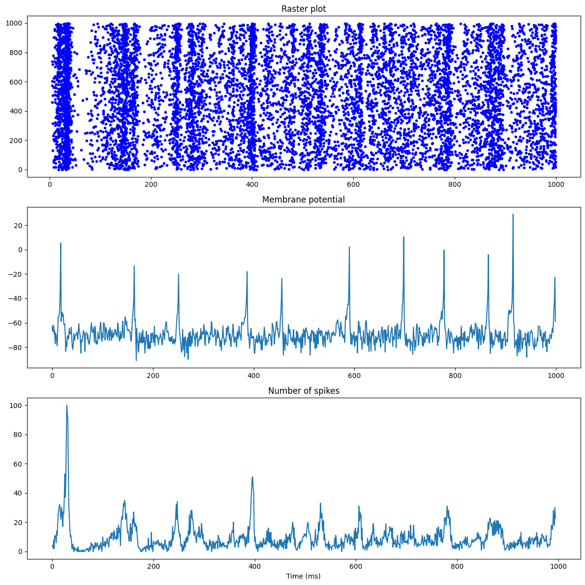

We can observe how the pusle-coupled network oscillates first at a low frequency, before emitting higher-frequency oscillations.