#!pip install ANNarchyBar Learning problem
![]()
![]()
The bar learning problem describes the process of learning receptive fields on an artificial input pattern. Images consisting of independent bars are used. Those images are generated as following: an 8*8 image can filled randomly by eight horizontal or vertical bars, with a probability of 1/8 for each.
These input images are fed into a neural population, whose neurons should learn to extract the independent components of the input distribution, namely single horizontal or vertical bars.
Model overview
The model consists of two populations inp and pop. The size of inp should be chosen to fit the input image size (here 8*8). The number of neurons in the pop population should be higher than the total number of independent bars (16, we choose here 32 neurons). The pop population gets excitory connections from inp through an all-to-all connection pattern. The same pattern is used for the inhibitory connections within pop.
Defining the neurons and populations
import numpy as np
import matplotlib.pyplot as plt

import ANNarchy as ann
ANNarchy 5.0 (5.0.2) on linux (posix).net = ann.Network()Input population:
The input pattern will be clamped into this population by the main loop for every trial, so we just need an InputArray to store the values:
N = 8
inp = net.create(ann.InputArray(geometry=(N, N)))
Learning population:
The neuron type composing this population sums up all the excitory inputs gain from inp and the lateral inhibition within pop.
\tau \frac {dr_{j}}{dt} + r_{j} = \sum_{i} w_{ij} \cdot r_{i}^{\text{inp}} - \sum_{k, k \ne j} w_{kj} * r_{k}
could be implemented as the following:
LeakyNeuron = ann.Neuron(
    parameters = dict(tau = 10.0),
    equations = ann.Variable("tau * dr/dt + r = sum(exc) - sum(inh)", min=0.0),
)
The firing rate is restricted to positive values with the min=0.0 attribute. The population of 32 neurons is created in the following way:
pop = net.create(geometry=(N, int(N/2)), neuron=LeakyNeuron)We define the population with a (8, 4) geometry for visualization only, its 2D structure does not influence computations at all. We could also use geometry=32 and reshape the array afterwards.
Defining the synapse and projections
Both feedforward (inp \rightarrow pop) and lateral (pop \rightarrow pop) projections are learned using the Oja learning rule (a regularized Hebbian learning rule ensuring the sum of all weights coming to a neuron is constant). Only some parameters will differ between the projections.
\tau \frac{dw_{ij}}{dt} = r_{i} \cdot r_{j} - \alpha \cdot r_{j}^{2} \cdot w_{ij}
where \alpha is a parameter defining the strength of the regularization, r_i is the pre-synaptic firing rate and r_j the post-synaptic one. The implementation of this synapse type is straightforward:
Oja = ann.Synapse(
    parameters = dict(
        tau = 2000.0,
        alpha = 8.0,
        min_w = 0.0,
    ),
    equations = ann.Variable(
        "tau * dw/dt = pre.r * post.r - alpha * post.r^2 * w",
        min='min_w'
    )
)
For this network we need to create two projections, one excitory between the populations inp and pop and one inhibitory within the pop population itself:
ff = net.connect(
    pre=inp,
    post=pop,
    target='exc',
    synapse = Oja
)
ff.all_to_all(
    weights = ann.Uniform(0.0, 0.5)
)

lat = net.connect(
    pre=pop,
    post=pop,
    target='inh',
    synapse = Oja
)
lat.all_to_all(
    weights = ann.Uniform(0.0, 1.0)
)
<ANNarchy.core.Projection.Projection at 0x7e7d5bf95d50>The two projections are all-to-all and use the Oja synapse type. They only differ by the parameter alpha (lower in pop):
lat.alpha = 0.3We can now compile the network:
net.compile()Compiling network 1... OKSetting inputs
Once the network is defined, one has to specify how inputs are fed into the inp population. A simple solution is to define a method that sets the firing rate of inp according to the specified probabilities every time it is called, and runs the simulation for 50 ms:
def trial():

    # Reset the firing rate for all neurons
    inp.r = 0.0

    # Clamp horizontal bars randomly
    hbars = np.random.binomial(n=1, p=1./N, size=N) == 1
    for i, exists in enumerate(hbars):
        inp[i, :].r = 1.0 if exists else inp[i, :].r

    # Clamp vertical bars randomly
    vbars = np.random.binomial(n=1, p=1./N, size=N) == 1
    for j, exists in enumerate(vbars):
        inp[:, j].r = 1.0 if exists else inp[:, j].r

    # Simulate for 50ms
    net.simulate(50.)

    # Return firing rates and receptive fields for visualization
    return inp.r, pop.r, ff.receptive_fields()
One can use here a single value or a Numpy array (e.g. np.zeros(inp.geometry))) to reset activity in inp, it does not matter.
For the random bars, we use the binomial distribution to decide for the existence of a vertical or horizontal bar with a probability of 1/8.
inp[i, :] and inp[:, j] are PopulationViews, i.e. groups of neurons defined by the sub-indices (here the rows and columns of inp). Their attributes, such as r, can be accessed and modified as if it were a regular population.
Running the simulation
Let’s have a look at the activities and receptive fields after one trial:
input_array, activity_array, weights = trial()from matplotlib.gridspec import GridSpec
fig = plt.figure(layout="constrained", figsize=(8, 8))
gs = GridSpec(2, 2, figure=fig)
ax1 = fig.add_subplot(gs[0, 0])
ax2 = fig.add_subplot(gs[0, 1])
ax3 = fig.add_subplot(gs[1, :])
im1 = ax1.imshow(input_array.T, interpolation='nearest', cmap=plt.cm.gray)
ax1.set_title('Input')
im2 = ax2.imshow(activity_array.T, interpolation='nearest', cmap=plt.cm.gray)
ax2.set_title('Feature')
im3 = ax3.imshow(weights.T, interpolation='nearest', cmap=plt.cm.gray, vmin=0.0, vmax=0.5)
ax3.set_title('Receptive fields')
fig.colorbar(im3)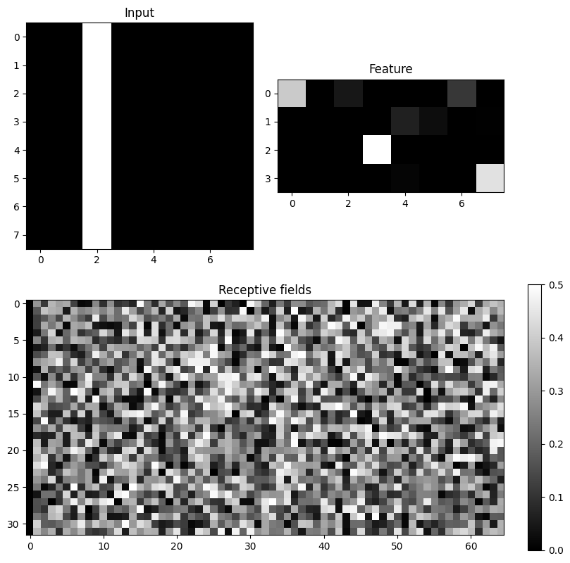
One or a few bars are present in inp, a few neurons react in pop, but the receptive fields are all random.
Let’s now define a for loop where the trial() method is called repetitively 10000 times:
inputs = []; features = []; rfs = []

T = 10000
for t in range(T):

    # Single trial
    input_r, feature_r, weights = trial()

    # Record every 10 trials
    if t % 10 == 0:
        inputs.append(input_r)
        features.append(feature_r)
        rfs.append(weights)
We can now visualize the activities and receptive fields after learning:
fig = plt.figure(layout="constrained", figsize=(8, 8))
gs = GridSpec(2, 2, figure=fig)
ax1 = fig.add_subplot(gs[0, 0])
ax2 = fig.add_subplot(gs[0, 1])
ax3 = fig.add_subplot(gs[1, :])

im1 = ax1.imshow(inputs[-1].T, interpolation='nearest', cmap=plt.cm.gray)
ax1.set_title('Input')
im2 = ax2.imshow(features[-1].T, interpolation='nearest', cmap=plt.cm.gray)
ax2.set_title('Feature')
im3 = ax3.imshow(rfs[-1].T, interpolation='nearest', cmap=plt.cm.gray, vmin=0.0, vmax=0.3)
ax3.set_title('Receptive fields')
fig.colorbar(im3)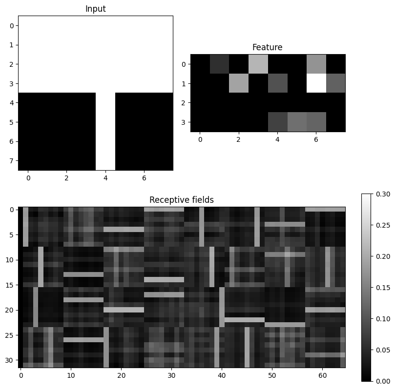
After 10000 trials, most neurons have developed a receptive field specific for a single horizontal or vertical bar, although these were always presented together.
Let’s now have a look at how these receptive fields develop over the course of training.
%matplotlib inline
from matplotlib import animation
from IPython.display import HTML

fig = plt.figure(layout="constrained", figsize=(8, 8))
gs = GridSpec(2, 2, figure=fig)
ax1 = fig.add_subplot(gs[0, 0])
ax2 = fig.add_subplot(gs[0, 1])
ax3 = fig.add_subplot(gs[1, :])

im1 = ax1.imshow(inputs[-1].T, interpolation='nearest', cmap=plt.cm.gray)
ax1.set_title('Input')
im2 = ax2.imshow(features[-1].T, interpolation='nearest', cmap=plt.cm.gray)
ax2.set_title('Feature')
im3 = ax3.imshow(rfs[-1].T, interpolation='nearest', cmap=plt.cm.gray, vmin=0.0, vmax=0.3)
ax3.set_title('Receptive fields')
cb = fig.colorbar(im3)

def drawframe(n):
    im1.set_data(inputs[n].T)
    im2.set_data(features[n].T)
    im3.set_data(rfs[n].T)
    return (im1, im2, im3)

anim = animation.FuncAnimation(fig, drawframe, frames=int(T/10), interval=20, blit=True)
plt.close()
HTML(anim.to_html5_video())Most neurons become selective for a single bar. However, due to the lateral inhibition, two neurons selective for the same bar will compete with each other. The “losing” neuron will have to modify its receptive field to let the winner have it. This explains the instability of some cells during learning.