#!pip install ANNarchyRecording BOLD signals - Davis model
![]()
![]()
import numpy as np

import ANNarchy as ann
import ANNarchy.extensions.bold as bold
ANNarchy 5.0 (5.0.2) on linux (posix).Davis model
Let’s now demonstrate how to define a custom BOLD model. The default Ballon model is defined by the following code:
balloon_RN = BoldModel(
    parameters = dict(
        phi       = 1.0         ,   kappa     = 1/1.54  ,
        gamma     = 1/2.46      ,   E_0       = 0.34    ,
        tau       = 0.98        ,   alpha     = 0.33    ,
        V_0       = 0.02        ,   v_0       = 40.3    ,
        TE        = 40/1000.    ,   epsilon   = 1.43    ,
        r_0       = 25.         ,   second    = 1000.0  ,
    ),
    equations = [
        # CBF input
        'I_CBF = sum(I_CBF)',
        'ds/dt = (phi * I_CBF - kappa * s - gamma * (f_in - 1))/second',
        ann.Variable('df_in/dt = s / second', init=1, min=0.01),

        # Balloon model
        ann.Variable('E  = 1 - (1 - E_0)**(1 / f_in)', init=0.3424),
        ann.Variable('dq/dt = (f_in * E / E_0 - (q / v) * f_out)/(tau*second)', init=1, min=0.01),
        ann.Variable('dv/dt = (f_in - f_out)/(tau*second)', init=1, min=0.01),
        ann.Variable('f_out = v**(1 / alpha)', init=1, min=0.01),

        # Revised coefficients
        'k_1 = 4.3 * v_0 * E_0 * TE',
        'k_2 = epsilon * r_0 * E_0 * TE',
        'k_3 = 1.0 - epsilon',

        # Non-linear BOLD equation
        'BOLD = V_0 * (k_1 * (1 - q) + k_2 * (1 - (q / v)) + k_3 * (1 - v))',
    ],
    inputs=['I_CBF']
)
It is very similar to the interface of a Neuron model, with parameters and equations defined in two multi-line strings. The input signal I_CBF has to be explicitly defined in the inputs argument to help the BOLD monitor create the mapping.
To demonstrate how to create a custom BOLD model, let’s suppose we want a model that computes both the BOLD signal of the Balloon model and the one of the Davis model:
Davis, T. L., Kwong, K. K., Weisskoff, R. M., and Rosen, B. R. (1998). Calibrated functional MRI: mapping the dynamics of oxidative metabolism. Proceedings of the National Academy of Sciences 95, 1834–1839
Without going into too many details, the Davis model computes the BOLD signal directly using f_in and E, without introducing a differential equation for the BOLD signal. Its implementation using the BOLD model would be:
DavisModel = BoldModel(
parameters = dict(
second = 1000.0,
phi = 1.0, # Friston et al. (2000)
kappa = 1/1.54,
gamma = 1/2.46,
E_0 = 0.34,
M = 0.149, # Griffeth & Buxton (2011)
alpha = 0.14,
beta = 0.91,
),
equations = [
# CBF-driving input as in Friston et al. (2000)
'I_CBF = sum(I_CBF)',
'ds/dt = (phi * I_CBF - kappa * s - gamma * (f_in - 1))/second',
ann.Variable('df_in/dt = s / second', init=1, min=0.01),
# Using part of the Balloon model to calculate r (normalized CMRO2) as in Buxton et al. (2004)
ann.Variable('E = 1 - (1 - E_0)**(1 / f_in)', init=0.34),
ann.Variable('r = f_in * E / E_0'),
# Davis model
'BOLD = M * (1 - f_in**alpha * (r / f_in)**beta)',
],
inputs=['I_CBF']
)Note that we could simply define two BOLD monitors using different models, but let’s create a complex model that does both for the sake of demonstration.
Let’s first redefine the populations of the previous notebook:
# Network
net = ann.Network()

# Two populations of 100 izhikevich neurons
pop1 = net.create(100, neuron=ann.Izhikevich)
pop2 = net.create(100, neuron=ann.Izhikevich)

# Set noise to create some baseline activity
pop1.noise = 5.0; pop2.noise = 5.0

# Compute mean firing rate in Hz on 100ms window
pop1.compute_firing_rate(window=100.0)
pop2.compute_firing_rate(window=100.0)

# Create required monitors
mon_pop1 = net.monitor(pop1, ["r"], start=False)
mon_pop2 = net.monitor(pop2, ["r"], start=False)
We can now create a hybrid model computing both the Balloon RN model of Stephan et al. (2007) and the Davis model:
balloon_Davis = bold.BoldModel(
    parameters = dict(
        phi       = 1.0         ,   kappa     = 1/1.54 ,
        gamma     = 1/2.46      ,   E_0       = 0.34   ,
        tau       = 0.98        ,   alpha     = 0.33   ,
        V_0       = 0.02        ,   v_0       = 40.3   ,
        TE        = 40/1000.    ,   epsilon   = 1.43   ,
        r_0       = 25.         ,   second    = 1000.0 ,
        M         = 0.062       ,   alpha2    = 0.14   ,
        beta      = 0.91
    ),
    equations = [

        # CBF input
        'I_CBF = sum(I_CBF)',
        'ds/dt = (phi * I_CBF - kappa * s - gamma * (f_in - 1))/second',
        ann.Variable('df_in/dt = s / second', init=1, min=0.01),

        # Balloon model
        ann.Variable('E  = 1 - (1 - E_0)**(1 / f_in)', init=0.3424),
        ann.Variable('dq/dt = (f_in * E / E_0 - (q / v) * f_out)/(tau*second)', init=1, min=0.01),
        ann.Variable('dv/dt = (f_in - f_out)/(tau*second)', init=1, min=0.01),
        ann.Variable('f_out = v**(1 / alpha)', init=1, min=0.01),

        # Revised coefficients
        'k_1 = 4.3 * v_0 * E_0 * TE',
        'k_2 = epsilon * r_0 * E_0 * TE',
        'k_3 = 1.0 - epsilon',

        # Non-linear BOLD equation
        'BOLD = V_0 * (k_1 * (1 - q) + k_2 * (1 - (q / v)) + k_3 * (1 - v))',

        # Davis model
        ann.Variable('r = f_in * E / E_0', init=1, min=0.01),
        'BOLD_Davis =  M * (1 - f_in**alpha2 * (r / f_in)**beta)',
    ],
    inputs=['I_CBF']
)
We now only need to pass that new object to the BOLD monitor, and specify that we want to record both BOLD and BOLD_Davis:
m_bold = net.boldmonitor(
# Recorded populations
populations = [pop1, pop2],
# BOLD model to use
bold_model = balloon_Davis,
# Mapping from pop.r to I_CBF
mapping = {'I_CBF': 'r'},
# Time window to compute the baseline.
normalize_input = 2000,
# Variables to be recorded
recorded_variables = ["I_CBF", "BOLD", "BOLD_Davis"],
)
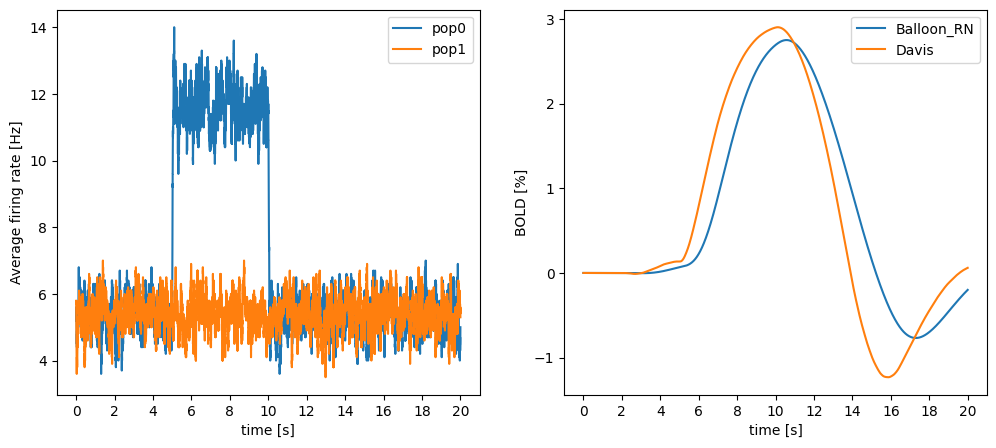
net.compile()Compiling network 1... OKWe run the same simulation protocol and compare the two BOLD signals. Note that the value of M has been modified to give a similar amplitude to both signals:
# Ramp up time
net.simulate(1000)

# Start recording
mon_pop1.start()
mon_pop2.start()
m_bold.start()

# we manipulate the noise for the half of the neurons
net.simulate(5000)      # 5s with low noise
pop1.noise = 7.5
net.simulate(5000)      # 5s with higher noise (one population)
pop1.noise = 5
net.simulate(10000)     # 10s with low noise

# retrieve the recordings
mean_fr1 = np.mean(mon_pop1.get("r"), axis=1)
mean_fr2 = np.mean(mon_pop2.get("r"), axis=1)

If_data = m_bold.get("I_CBF")
bold_data = m_bold.get("BOLD")
davis_data = m_bold.get("BOLD_Davis")
import matplotlib.pyplot as plt
plt.figure(figsize=(12, 5))
# mean firing rate
ax1 = plt.subplot(121)
ax1.plot(mean_fr1, label="pop0")
ax1.plot(mean_fr2, label="pop1")
plt.legend()
ax1.set_ylabel("Average firing rate [Hz]")
# BOLD input signal as percent
ax2 = plt.subplot(122)
ax2.plot(bold_data*100.0, label="Balloon_RN")
ax2.plot(davis_data*100.0, label="Davis")
plt.legend()
ax2.set_ylabel("BOLD [%]")
# x-axis labels as seconds
for ax in [ax1, ax2]:
ax.set_xticks(np.arange(0,21,2)*1000)
ax.set_xticklabels(np.arange(0,21,2))
ax.set_xlabel("time [s]")
plt.show()