#!pip install ANNarchyMiconi network
![]()
![]()
Reward-modulated recurrent network based on:
Miconi T. (2017). Biologically plausible learning in recurrent neural networks reproduces neural dynamics observed during cognitive tasks. eLife 6:e20899. doi:10.7554/eLife.20899
import numpy as np
import matplotlib.pyplot as plt

#Less "spamy" progress bar but requires additionally ipywidgets
from tqdm.notebook import tqdm
#from tqdm import tqdm

import ANNarchy as ann
ANNarchy 5.0 (5.0.2) on linux (posix).Each neuron in the reservoir follows the following equations:
\tau \frac{dx(t)}{dt} + x(t) = \sum_\text{input} W^\text{IN} \, r^\text{IN}(t) + \sum_\text{rec} W^\text{REC} \, r(t) + \xi(t)
r(t) = \tanh(x(t))
where \xi(t) is a random perturbation at 3 Hz, with an amplitude randomly sampled between -A and +A.
We additionally keep track of the mean firing rate with a sliding average:
\tilde{x}(t) = \alpha \, \tilde{x}(t) + (1 - \alpha) \, x(t)
The three first neurons keep a constant rate throughout learning (1 or -1) to provide some bias to the other neurons.
neuron = ann.Neuron(
    parameters = dict(
        tau = 30.0, # Time constant
        constant = ann.Parameter(0.0, locality='local'), # The four first neurons have constant rates
        alpha = 0.05, # To compute the sliding mean
        f = 3.0, # Frequency of the perturbation
        A = 16., # Perturbation amplitude. dt*A/tau should be 0.5...
    ),
    equations = [
        # Perturbation
        'perturbation = if Uniform(0.0, 1.0) < f/1000.: 1.0 else: 0.0',
        'noise = if perturbation > 0.5: A * Uniform(-1.0, 1.0) else: 0.0',

        # ODE for x
        'x += dt*(sum(in) + sum(exc) - x + noise)/tau',

        # Output r
        'rprev = r', # store r at previous time step
        'r = if constant == 0.0: tanh(x) else: tanh(constant)',

        # Sliding mean
        'delta_x = x - x_mean',
        'x_mean = alpha * x_mean + (1 - alpha) * x',
    ]
)
The learning rule is defined by a trace e_{i, j}(t) for each synapse i \rightarrow j incremented at each time step with:
e_{i, j}(t) = e_{i, j}(t-1) + (r_i (t) \, x_j(t))^3
At the end T of a trial, the reward R is delivered and all weights are updated using:
\Delta w_{i, j} = \eta \, e_{i, j}(T) \, |R_\text{mean}| \, (R - R_\text{mean})
where R_\text{mean} is the mean reward for the task. Here the reward is defined as the opposite of the prediction error.
All traces are then reset to 0 for the next trial. Weight changes are clamped between -0.0003 and 0.0003.
As ANNarchy applies the synaptic equations at each time step, we need to introduce a global boolean learning_phase which performs trace integration when false, and allows weight update when true.
synapse = ann.Synapse(
    parameters=dict(
        eta = 0.5, # Learning rate
        max_weight_change = 0.0003, # Clip the weight changes

        # Flag to allow learning only at the end of a trial
        learning_phase = ann.Parameter(False, 'global', 'bool'),
        reward = 0.0, # Reward received
        mean_reward = 0.0, # Mean Reward received
    ),
    equations = [
        # Trace
        """
        trace += if not(learning_phase):
                    power(pre.rprev * (post.delta_x), 3)
                 else:
                    0.0
        """,

        # Weight update only at the end of the trial
        ann.Variable("""
            delta_w = if learning_phase:
                    eta * trace * fabs(mean_reward) * (reward - mean_reward)
                else:
                    0.0
        """,
        min='-max_weight_change', max='max_weight_change'),

        # Weight update
        "w += delta_w",

    ]
)
We implement the network as a class deriving from ann.Network. The network has two inputs A and B, so we create the corresponding static population. The reservoir has 200 neurons, 3 of which having constant rates to serve as biases for the other neurons.
Input weights are uniformly distributed between -1 and 1.
The recurrent weights are normally distributed, with a coupling strength of g=1.5 (edge of chaos). In the original paper, the projection is fully connected (but self-connections are avoided). Using a sparse (0.1) connectivity matrix leads to similar results and is much faster.
class MiconiNetwork (ann.Network):

    def __init__(self, N, g, sparseness):

        # Input population
        self.inp = self.create(2, ann.Neuron("r=0.0"))

        # Recurrent population
        self.pop = self.create(N, neuron)

        # Biases
        self.pop[0].constant = 1.0
        self.pop[1].constant = 1.0
        self.pop[2].constant = -1.0

        # Input weights
        self.Wi = self.connect(self.inp, self.pop, 'in')
        self.Wi.all_to_all(weights=ann.Uniform(-1.0, 1.0))

        # Recurrent weights
        self.Wrec = self.connect(self.pop, self.pop, 'exc', synapse)
        if sparseness == 1.0:
            self.Wrec.all_to_all(weights=ann.Normal(0., g/np.sqrt(N)))
        else:
            self.Wrec.fixed_probability(
                probability=sparseness,
                weights=ann.Normal(0., g/np.sqrt(sparseness*N))
            )

        # Monitor
        self.m = self.monitor(self.pop, ['r'], start=False)
net = MiconiNetwork(N=200, g=1.5, sparseness=0.1)
net.compile()Compiling network 1... OKThe output of the reservoir is chosen to be the neuron of index 100.
OUTPUT_NEURON = 100Parameters defining the task:
# Durations
d_stim = 200
d_delay= 200
d_response = 200
Definition of a DNMS trial (AA, AB, BA, BB):
def dnms_trial(trial_number, input, target, R_mean, record=False, perturbation=True):

    # Switch off perturbations if needed
    if not perturbation:
        old_A = net.pop.A
        net.pop.A = 0.0

    # Reinitialize network
    net.pop.x = ann.Uniform(-0.1, 0.1).get_values(net.pop.size)
    net.pop.r = np.tanh(net.pop.x)
    net.pop[0].r = np.tanh(1.0)
    net.pop[1].r = np.tanh(1.0)
    net.pop[2].r = np.tanh(-1.0)

    if record: net.m.resume()

    # First input
    net.inp[input[0]].r = 1.0
    net.simulate(d_stim)

    # Delay
    net.inp.r = 0.0
    net.simulate(d_delay)

    # Second input
    net.inp[input[1]].r = 1.0
    net.simulate(d_stim)

    # Delay
    net.inp.r = 0.0
    net.simulate(d_delay)

    # Response
    if not record: net.m.resume()
    net.inp.r = 0.0
    net.simulate(d_response)

    # Read the output
    net.m.pause()
    recordings = net.m.get('r')

    # Response is over the last 200 ms
    output = recordings[-int(d_response):, OUTPUT_NEURON] # neuron 100 over the last 200 ms

    # Compute the reward as the opposite of the absolute error
    reward = - np.mean(np.abs(target - output))

    # The first 25 trial do not learn, to let R_mean get realistic values
    if trial_number > 25:

        # Apply the learning rule
        net.Wrec.learning_phase = True
        net.Wrec.reward = reward
        net.Wrec.mean_reward = R_mean

        # Learn for one step
        net.step()

        # Reset the traces
        net.Wrec.learning_phase = False
        net.Wrec.trace = 0.0
        #_ = m.get() # to flush the recording of the last step

    # Switch back on perturbations if needed
    if not perturbation:
        net.pop.A = old_A

    return recordings, reward
Let’s visualize the activity of the output neuron during the first four trials.
# Perform the four different trials successively
initialAA, errorAA = dnms_trial(0, [0, 0], -0.98, 0.0, record=True)
initialAB, errorAB = dnms_trial(0, [0, 1], +0.98, 0.0, record=True)
initialBA, errorBA = dnms_trial(0, [1, 0], +0.98, 0.0, record=True)
initialBB, errorBB = dnms_trial(0, [1, 1], -0.98, 0.0, record=True)

plt.figure(figsize=(12, 10))
ax = plt.subplot(221)
ax.plot(initialAA[:, OUTPUT_NEURON])
ax.set_ylim((-1., 1.))
ax.set_title('Output AA -1')
ax = plt.subplot(222)
ax.plot(initialBA[:, OUTPUT_NEURON])
ax.set_ylim((-1., 1.))
ax.set_title('Output BA +1')
ax = plt.subplot(223)
ax.plot(initialAB[:, OUTPUT_NEURON])
ax.set_ylim((-1., 1.))
ax.set_title('Output AB +1')
ax = plt.subplot(224)
ax.plot(initialBB[:, OUTPUT_NEURON])
ax.set_ylim((-1., 1.))
ax.set_title('Output BB -1')
plt.show()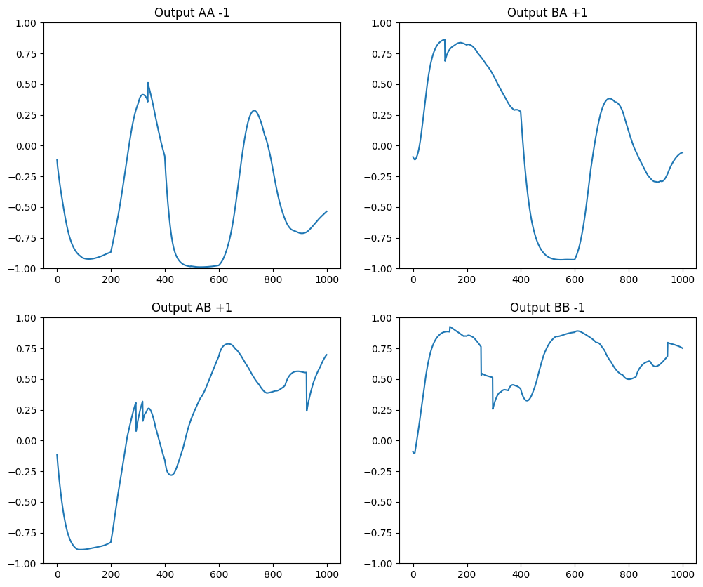
We can now run the simulation for 1500 trials. Beware, this can take 15 to 20 minutes.
# Compute the mean reward per trial
R_mean = - np.ones((2, 2))
alpha = 0.75

# Many trials of each type
record_rewards = []

for trial in (t := tqdm(range(10000))):

    # Perform the four different trials successively
    _, rewardAA = dnms_trial(trial, [0, 0], -0.98, R_mean[0, 0])

    _, rewardAB = dnms_trial(trial, [0, 1], +0.98, R_mean[0, 1])

    _, rewardBA = dnms_trial(trial, [1, 0], +0.98, R_mean[1, 0])

    _, rewardBB = dnms_trial(trial, [1, 1], -0.98, R_mean[1, 1])

    # Reward
    reward = np.array([[rewardAA, rewardBA], [rewardBA, rewardBB]])

    # Update mean reward
    R_mean = alpha * R_mean + (1.- alpha) * reward

    record_rewards.append(R_mean)
    t.set_description(
        f'AA: {R_mean[0, 0]:.2f} AB: {R_mean[0, 1]:.2f} BA: {R_mean[1, 0]:.2f} BB: {R_mean[1, 1]:.2f}'
    )
record_rewards = np.array(record_rewards)
plt.figure(figsize=(10, 6))
plt.plot(record_rewards[:, 0, 0], label='AA')
plt.plot(record_rewards[:, 0, 1], label='AB')
plt.plot(record_rewards[:, 1, 0], label='BA')
plt.plot(record_rewards[:, 1, 1], label='BB')
plt.plot(record_rewards.mean(axis=(1,2)), label='mean')
plt.xlabel("Trials")
plt.ylabel("Mean reward")
plt.legend()
plt.show()
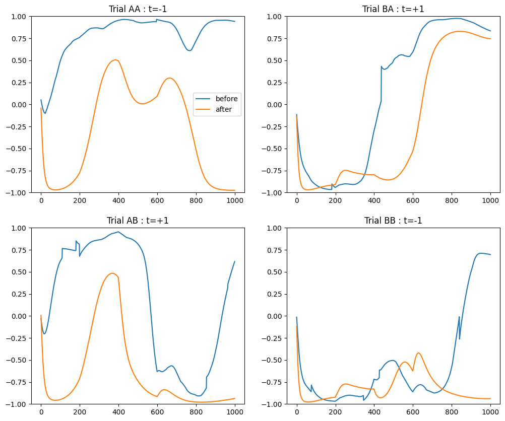
# Perform the four different trials without perturbation for testing
recordsAA, errorAA = dnms_trial(0, [0, 0], -0.98, 0.0, record=True, perturbation=False)
recordsAB, errorAB = dnms_trial(0, [0, 1], +0.98, 0.0, record=True, perturbation=False)
recordsBA, errorBA = dnms_trial(0, [1, 0], +0.98, 0.0, record=True, perturbation=False)
recordsBB, errorBB = dnms_trial(0, [1, 1], -0.98, 0.0, record=True, perturbation=False)

plt.figure(figsize=(12, 10))
plt.subplot(221)
plt.plot(initialAA[:, OUTPUT_NEURON], label='before')
plt.plot(recordsAA[:, OUTPUT_NEURON], label='after')
plt.legend()
plt.ylim((-1., 1.))
plt.title('Trial AA : t=-1')
plt.subplot(222)
plt.plot(initialBA[:, OUTPUT_NEURON], label='before')
plt.plot(recordsBA[:, OUTPUT_NEURON], label='after')
plt.ylim((-1., 1.))
plt.title('Trial BA : t=+1')
plt.subplot(223)
plt.plot(initialAB[:, OUTPUT_NEURON], label='before')
plt.plot(recordsAB[:, OUTPUT_NEURON], label='after')
plt.ylim((-1., 1.))
plt.title('Trial AB : t=+1')
plt.subplot(224)
plt.plot(initialBB[:, OUTPUT_NEURON], label='before')
plt.plot(recordsBB[:, OUTPUT_NEURON], label='after')
plt.ylim((-1., 1.))
plt.title('Trial BB : t=-1')
plt.show()