Logging with tensorboard

The tensorboard extension allows to visualize ANNarchy simulations using tensorboard. It requires the tensorboardX package:

pip install tensorboardX

The Logger class is a thin wrapper around tensorboardX.SummaryWriter, which you could also use directly. The doc is available at https://tensorboardx.readthedocs.io. Tensorboard can read any logging data, as long as they are saved in the right format (tfevents), so it is not limited to tensorflow. TensorboardX has been developed to allow the use of tensorboard with pytorch.

The extension has to be imported explicitly:

import ANNarchy as ann
from ANNarchy.extensions.tensorboard import Logger

For detailed examples of how to use the extension, refer to the examples Basal Ganglia and Bayesian optimization, which are available as notebooks in the folder examples/tensorboard.

Creating the logger

The Logger class has to be closed properly at the end of the script, so it is advised to use a context:

with ann.Logger() as logger:
    logger.add_scalar("Accuracy", acc, trial)

You can also make sure to close it:

logger = ann.Logger()
logger.add_scalar("Accuracy", acc, trial)
logger.close()

By default, the logs will be written in a subfolder of ./runs/ (which will be created in the current directory). The subfolder is a combination of the current datetime and of the hostname, e.g. ./runs/Apr22_12-11-22_machine. You can control these two elements by passing arguments to Logger():

with ann.Logger(logdir="/tmp/annarchy", experiment="trial1"): # logs in /tmp/annarchy/trial1

Launching tensorboard

After (or while) logging data within your simulation, run tensorboard in the terminal by specifying the path to the log directory:

tensorboard --logdir runs

You will then be asked to open localhost:6006 in your browser and will see a page similar to this:

Structure of a neural network

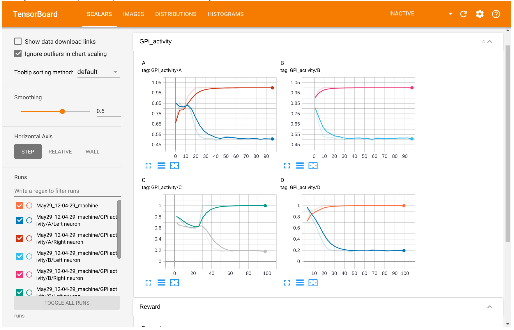
The information logged will be available in the different tabs (scalars, images...). You can also visualize and compare several experiments at the same time.

Logging scalars

The add_* methods allow you to log various structures, such as scalars, images, histograms, figures, etc.

The simplest information to log is a scalar, for example the accuracy at the end of a trial:

with ann.Logger() as logger:
    for trial in range(100):
        ann.simulate(1000.0)
        accuracy = ...
        logger.add_scalar("Accuracy", accuracy, trial)

A tag should be given for each plot as the first argument. In the example above, the figure with the accuracy will be labelled "Accuracy" in tensorboard. You can also group plots together with 2-levels tags such as:

with ann.Logger() as logger:
    for trial in range(100):
        ann.simulate(1000.0)
        train_accuracy = ...
        test_accuracy = ...
        logger.add_scalar("Accuracy/Train", train_accuracy, trial)
        logger.add_scalar("Accuracy/Test", test_accuracy, trial)

The second argument is the scalar, obviously. The third is the index of x-axis of the plot. It can be the index of the trial, the current time or whatever you prefer.

If you want to display several scalars on the same plot, you can use the method add_scalars() and provide a dictionary:

with ann.Logger() as logger:
    for trial in range(100):
        ann.simulate(1000.0)
        train_accuracy = ...
        test_accuracy = ...
        logger.add_scalars("Accuracy", {'train': train_accuracy, 'test': test_accuracy}, trial)

Logging images

It is also possible to log images, for example an input image or the firing rate of a 2D population, with the add_image() method:

with ann.Logger() as logger:
    for trial in range(100):
        ann.simulate(1000.0)
        img = pop.r.reshape((10, 10))
        logger.add_image("Population/Firing rate", img, trial)

The image must be a numpy array of size (height, width) for monochrome images or (height, width, 3) for colored images.

The values must be floats between 0 and 1 or integers between 0 and 255 in order to be displayed correctly. You can either do it yourself, or pass equalize=True to the add_image():

logger.add_image("Population/Firing rate", img, trial, equalize=True)

The min/max values in the array are internally used to rescale the image:

img = (img - img.min())/(img.max() - img.min())

To display several images together, for example the receptive fields of a population, an array of size (number, height, width) or (number, height, width, 3) can be passed to add_images(), where number is the number of images to display:

with ann.Logger() as logger:
    for trial in range(100):
        ann.simulate(1000.0)
        weights= proj.w.reshape(100, 10, 10) # 100 post neurons, 10*10 pre neurons
        logger.add_images("Projection/Receptive fields", weights, trial, equalize=True)

equalize=True applies the same scaling to all images, but you additionally pass equalize_per_image=True to have indepent scalings per image.

Logging histograms

Histograms can also be logged, for example to visualize the statistics of weights in a projection:

with ann.Logger() as logger:
    for trial in range(100):
        ann.simulate(1000.0)
        weights= proj.w.flatten()
        logger.add_histogram("Weight distribution", weights, trial)

Logging figures

Matplotlib figures can also be logged:

with ann.Logger() as logger:
    for trial in range(100):
        ann.simulate(1000.0)
        fig = plt.figure()
        plt.plot(pop.r)
        logger.add_figure("Activity", fig, trial)

add_figure() will automatically close the figure, no need to call show().

Beware that this is very slow and requires a lot of space.

Logging parameters

The previous methods can be called multiple times during a simulation, in order to visualize the changes during learning.

add_parameters() is more useful in the context of hyperparameter optimization, where the same network with different parameters is run multiple times.

Only once per simulation, typically at the end, you can log the value of some important parameters together with some metrics such as accuracy, error rate or so. This will allow tensorboard to display over multiple runs the relation between the parameters and the metrics in the tab “HPARAMS”:

with ann.Logger() as logger:
    # ...
    logger.add_parameters({'learning_rate': lr, 'tau': tau}, {'accuracy': accuracy}) 

Refer to Bayesian optimization for an example using the hyperopt library.