#!pip install ANNarchyANN-to-SNN conversion - MLP
![]()
![]()
This notebook demonstrates how to transform a fully-connected neural network trained using tensorflow/keras into an SNN network usable in ANNarchy.
The methods are adapted from the original models used in:
Diehl et al. (2015) “Fast-classifying, high-accuracy spiking deep networks through weight and threshold balancing” Proceedings of IJCNN. doi: 10.1109/IJCNN.2015.7280696
import numpy as np
import matplotlib.pyplot as plt

import tensorflow as tf
print(f"Tensorflow {tf.__version__}")
Tensorflow 2.16.2First we need to download and process the MNIST dataset provided by tensorflow.
# Download data
(X_train, t_train), (X_test, t_test) = tf.keras.datasets.mnist.load_data()

# Normalize inputs
X_train = X_train.reshape(X_train.shape[0], 784).astype('float32') / 255.
X_test = X_test.reshape(X_test.shape[0], 784).astype('float32') / 255.

# One-hot output vectors
T_train = tf.keras.utils.to_categorical(t_train, 10)
T_test = tf.keras.utils.to_categorical(t_test, 10)
Training an ANN in tensorflow/keras
The tensorflow.keras network is build using the functional API.
The fully-connected network has two fully connected layers with ReLU, no bias, dropout at 0.5, and a softmax output layer with 10 neurons. We use the standard SGD optimizer and the categorical crossentropy loss for classification.
def create_mlp():
    # Model
    inputs = tf.keras.layers.Input(shape=(784,))
    x= tf.keras.layers.Dense(128, use_bias=False, activation='relu')(inputs)
    x = tf.keras.layers.Dropout(0.5)(x)
    x= tf.keras.layers.Dense(128, use_bias=False, activation='relu')(x)
    x = tf.keras.layers.Dropout(0.5)(x)
    x=tf.keras.layers.Dense(10, use_bias=False, activation='softmax')(x)

    model= tf.keras.Model(inputs, x)

    # Optimizer
    optimizer = tf.keras.optimizers.SGD(learning_rate=0.05)

    # Loss function
    model.compile(
        loss='categorical_crossentropy', # loss function
        optimizer=optimizer, # learning rule
        metrics=['accuracy'] # show accuracy
    )
    print(model.summary())

    return model
We can now train the network and save the weights in the HDF5 format.
# Create model
model = create_mlp()

# Train model
history = model.fit(
    X_train, T_train,       # training data
    batch_size=128,          # batch size
    epochs=20,              # Maximum number of epochs
    validation_split=0.1,   # Percentage of training data used for validation
)

model.save("runs/mlp.keras")

# Test model
predictions_keras = model.predict(X_test, verbose=0)
test_loss, test_accuracy = model.evaluate(X_test, T_test, verbose=0)
print(f"Test accuracy: {test_accuracy}")
Model: "functional"
┏━━━━━━━━━━━━━━━━━━━━━━━━━━━━━━━━━┳━━━━━━━━━━━━━━━━━━━━━━━━┳━━━━━━━━━━━━━━━┓
┃ Layer (type)                    ┃ Output Shape           ┃       Param # ┃
┡━━━━━━━━━━━━━━━━━━━━━━━━━━━━━━━━━╇━━━━━━━━━━━━━━━━━━━━━━━━╇━━━━━━━━━━━━━━━┩
│ input_layer (InputLayer)        │ (None, 784)            │             0 │
├─────────────────────────────────┼────────────────────────┼───────────────┤
│ dense (Dense)                   │ (None, 128)            │       100,352 │
├─────────────────────────────────┼────────────────────────┼───────────────┤
│ dropout (Dropout)               │ (None, 128)            │             0 │
├─────────────────────────────────┼────────────────────────┼───────────────┤
│ dense_1 (Dense)                 │ (None, 128)            │        16,384 │
├─────────────────────────────────┼────────────────────────┼───────────────┤
│ dropout_1 (Dropout)             │ (None, 128)            │             0 │
├─────────────────────────────────┼────────────────────────┼───────────────┤
│ dense_2 (Dense)                 │ (None, 10)             │         1,280 │
└─────────────────────────────────┴────────────────────────┴───────────────┘
Total params: 118,016 (461.00 KB)
Trainable params: 118,016 (461.00 KB)
Non-trainable params: 0 (0.00 B)
None

Epoch 1/20

422/422 ━━━━━━━━━━━━━━━━━━━━ 1s 2ms/step - accuracy: 0.4837 - loss: 1.5160 - val_accuracy: 0.9123 - val_loss: 0.3443

Epoch 2/20

422/422 ━━━━━━━━━━━━━━━━━━━━ 1s 1ms/step - accuracy: 0.8178 - loss: 0.5996 - val_accuracy: 0.9310 - val_loss: 0.2473

Epoch 3/20

422/422 ━━━━━━━━━━━━━━━━━━━━ 1s 1ms/step - accuracy: 0.8566 - loss: 0.4747 - val_accuracy: 0.9405 - val_loss: 0.2079

Epoch 4/20

422/422 ━━━━━━━━━━━━━━━━━━━━ 1s 1ms/step - accuracy: 0.8771 - loss: 0.4162 - val_accuracy: 0.9492 - val_loss: 0.1831

Epoch 5/20

422/422 ━━━━━━━━━━━━━━━━━━━━ 1s 1ms/step - accuracy: 0.8934 - loss: 0.3715 - val_accuracy: 0.9532 - val_loss: 0.1676

Epoch 6/20

422/422 ━━━━━━━━━━━━━━━━━━━━ 1s 1ms/step - accuracy: 0.8999 - loss: 0.3453 - val_accuracy: 0.9588 - val_loss: 0.1531

Epoch 7/20

422/422 ━━━━━━━━━━━━━━━━━━━━ 1s 2ms/step - accuracy: 0.9066 - loss: 0.3198 - val_accuracy: 0.9612 - val_loss: 0.1427

Epoch 8/20

422/422 ━━━━━━━━━━━━━━━━━━━━ 1s 1ms/step - accuracy: 0.9113 - loss: 0.3056 - val_accuracy: 0.9648 - val_loss: 0.1340

Epoch 9/20

422/422 ━━━━━━━━━━━━━━━━━━━━ 1s 1ms/step - accuracy: 0.9183 - loss: 0.2816 - val_accuracy: 0.9648 - val_loss: 0.1290

Epoch 10/20

422/422 ━━━━━━━━━━━━━━━━━━━━ 1s 1ms/step - accuracy: 0.9229 - loss: 0.2682 - val_accuracy: 0.9653 - val_loss: 0.1226

Epoch 11/20

422/422 ━━━━━━━━━━━━━━━━━━━━ 1s 1ms/step - accuracy: 0.9225 - loss: 0.2673 - val_accuracy: 0.9678 - val_loss: 0.1180

Epoch 12/20

422/422 ━━━━━━━━━━━━━━━━━━━━ 1s 1ms/step - accuracy: 0.9239 - loss: 0.2624 - val_accuracy: 0.9683 - val_loss: 0.1135

Epoch 13/20

422/422 ━━━━━━━━━━━━━━━━━━━━ 1s 1ms/step - accuracy: 0.9272 - loss: 0.2503 - val_accuracy: 0.9693 - val_loss: 0.1106

Epoch 14/20

422/422 ━━━━━━━━━━━━━━━━━━━━ 1s 1ms/step - accuracy: 0.9281 - loss: 0.2475 - val_accuracy: 0.9695 - val_loss: 0.1103

Epoch 15/20

422/422 ━━━━━━━━━━━━━━━━━━━━ 1s 1ms/step - accuracy: 0.9319 - loss: 0.2331 - val_accuracy: 0.9712 - val_loss: 0.1040

Epoch 16/20

422/422 ━━━━━━━━━━━━━━━━━━━━ 1s 1ms/step - accuracy: 0.9368 - loss: 0.2208 - val_accuracy: 0.9713 - val_loss: 0.1031

Epoch 17/20

422/422 ━━━━━━━━━━━━━━━━━━━━ 1s 1ms/step - accuracy: 0.9369 - loss: 0.2183 - val_accuracy: 0.9720 - val_loss: 0.1028

Epoch 18/20

422/422 ━━━━━━━━━━━━━━━━━━━━ 1s 1ms/step - accuracy: 0.9352 - loss: 0.2153 - val_accuracy: 0.9737 - val_loss: 0.1000

Epoch 19/20

422/422 ━━━━━━━━━━━━━━━━━━━━ 1s 1ms/step - accuracy: 0.9426 - loss: 0.2030 - val_accuracy: 0.9737 - val_loss: 0.0971

Epoch 20/20

422/422 ━━━━━━━━━━━━━━━━━━━━ 1s 1ms/step - accuracy: 0.9430 - loss: 0.2052 - val_accuracy: 0.9727 - val_loss: 0.0987

Test accuracy: 0.9652000069618225
plt.figure(figsize=(12, 6))
plt.subplot(121)
plt.plot(history.history['loss'], '-r', label="Training")
plt.plot(history.history['val_loss'], '-b', label="Validation")
plt.xlabel('Epoch #')
plt.ylabel('Loss')
plt.legend()

plt.subplot(122)
plt.plot(history.history['accuracy'], '-r', label="Training")
plt.plot(history.history['val_accuracy'], '-b', label="Validation")
plt.xlabel('Epoch #')
plt.ylabel('Accuracy')
plt.legend()
plt.show()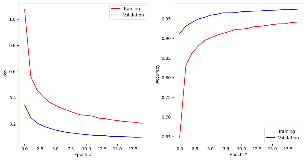
Initialize the ANN-to-SNN converter
We first create an instance of the ANN-to-SNN conversion object. The function receives the input_encoding parameter, which is the type of input encoding we want to use.
By default, there are intrinsically bursting (IB), phase shift oscillation (PSO) and Poisson (poisson) available.
from ANNarchy.extensions.ann_to_snn_conversion import ANNtoSNNConverter

snn_converter = ANNtoSNNConverter(
    input_encoding='IB',
    hidden_neuron='IaF',
    read_out='spike_count',
)
ANNarchy 4.8 (4.8.3) on darwin (posix).After that, we provide the TensorFlow model stored as a .keras file to the conversion tool. The print-out of the network structure of the imported network is suppressed when show_info=False is provided to load_keras_model.
net = snn_converter.load_keras_model("runs/mlp.keras", show_info=True)WARNING: Dense representation is an experimental feature for spiking models, we greatly appreciate bug reports.
* Input layer: input_layer, (784,)
* InputLayer skipped.
* Dense layer: dense, 128
weights: (128, 784)
mean -0.0038075943011790514, std 0.05276760458946228
min -0.32009223103523254, max 0.24077153205871582
* Dropout skipped.
* Dense layer: dense_1, 128
weights: (128, 128)
mean 0.0048642707988619804, std 0.10200534760951996
min -0.2624298334121704, max 0.4079423248767853
* Dropout skipped.
* Dense layer: dense_2, 10
weights: (10, 128)
mean -0.0005833255127072334, std 0.21552757918834686
min -0.5742316246032715, max 0.4535660445690155
When the network has been built successfully, we can perform a test using all MNIST training samples. Using duration_per_sample, the duration simulated for each image can be specified. Here, 200 ms seem to be enough.
predictions_snn = snn_converter.predict(X_test, duration_per_sample=200) 0%| | 0/10000 [00:00<?, ?it/s]100%|██████████| 10000/10000 [00:54<00:00, 182.00it/s]Using the recorded predictions, we can now compute the accuracy using scikit-learn for all presented samples.
from sklearn.metrics import classification_report, accuracy_score

print(classification_report(t_test, predictions_snn))
print("Test accuracy of the SNN:", accuracy_score(t_test, predictions_snn))
precision recall f1-score support
0 0.97 0.99 0.98 980
1 0.98 0.98 0.98 1135
2 0.96 0.97 0.96 1032
3 0.94 0.97 0.95 1010
4 0.97 0.95 0.96 982
5 0.97 0.94 0.95 892
6 0.96 0.97 0.97 958
7 0.96 0.96 0.96 1028
8 0.96 0.94 0.95 974
9 0.96 0.95 0.95 1009
accuracy 0.96 10000
macro avg 0.96 0.96 0.96 10000
weighted avg 0.96 0.96 0.96 10000
Test accuracy of the SNN: 0.9623For comparison, here is the performance of the original ANN in keras:
print(classification_report(t_test, predictions_keras.argmax(axis=1)))
print("Test accuracy of the ANN:", accuracy_score(t_test, predictions_keras.argmax(axis=1)))
precision recall f1-score support
0 0.97 0.98 0.98 980
1 0.98 0.99 0.98 1135
2 0.96 0.97 0.96 1032
3 0.94 0.97 0.96 1010
4 0.96 0.96 0.96 982
5 0.97 0.95 0.96 892
6 0.96 0.97 0.97 958
7 0.97 0.97 0.97 1028
8 0.97 0.94 0.96 974
9 0.97 0.94 0.96 1009
accuracy 0.97 10000
macro avg 0.97 0.96 0.96 10000
weighted avg 0.97 0.97 0.97 10000
Test accuracy of the ANN: 0.9652